Model: how it works
The QUANTUM AQUA predictive engine operates by modeling groundwater as a complex, dynamic system influenced by interactions among geospatial, climatic, geological, hydrological, and satellite-derived variables. Conceptually, the model follows a quantum-inspired computational framework, allowing it to represent nonlinear relationships, uncertainty, and spatiotemporal evolution in ways that traditional approaches cannot. Its formulation draws on principles related to the time-dependent Schrödinger equation, enabling the engine to capture how multiple environmental factors interact and propagate over time within groundwater systems.
The system integrates diverse data sources—optical imagery, SAR measurements, GRACE gravity signals, topography, geology, and climate indicators—into a unified predictive structure capable of delivering high-resolution, actionable intelligence.
Quantum Aqua is a 4D system, meaning it can analyze groundwater across space and time simultaneously. This ability allows the system to “see” beneath the surface in ways traditional models cannot.
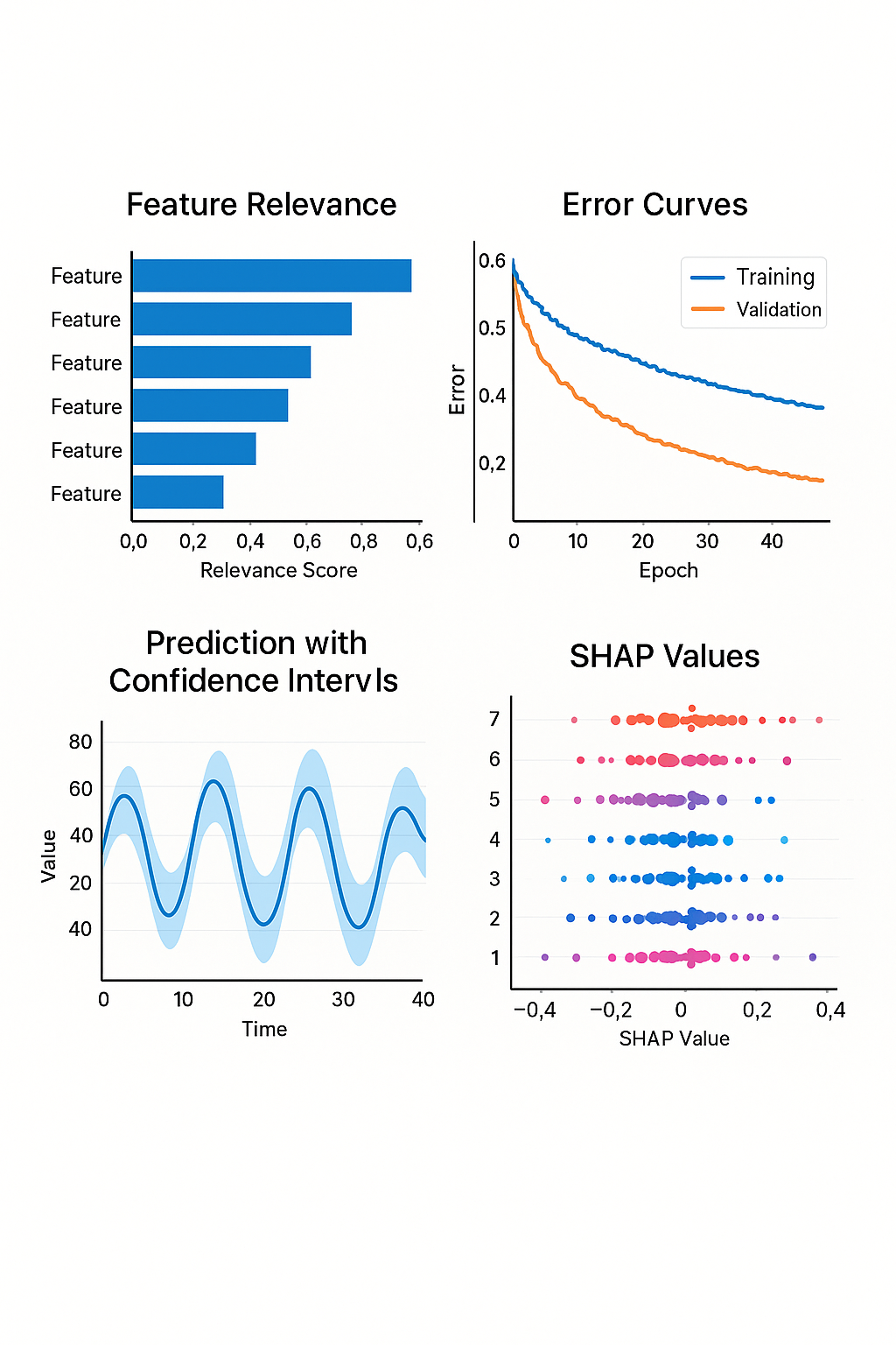
This figure presents key diagnostic outputs of the Quantum Aqua predictive engine: feature relevance scores identifying influential variables, training and validation error curves showing model convergence, prediction traces with confidence intervals illustrating uncertainty, and SHAP value distributions providing input–output interpretability.


The QUANTUM AQUA engine is a proprietary and patented technology. Its internal mechanics, including equations, solvers, architecture, parameterization, and computational pipeline, are strictly protected as an industrial trade secret, and therefore cannot be publicly disclosed. Next, we present several widely used metrics that help evaluate model efficiency and predictive performance.

Feature Relevance. Shows how much each input variable contributes to the model’s final prediction. It ranks variables by importance, highlighting which satellite, geological, climatic, or topographic features have the strongest influence on groundwater behavior.
Error Curves. Illustrate how the model’s prediction error evolves during training. They help assess model stability, convergence, and potential overfitting by comparing training error vs. validation error over multiple epochs.
Confidence Intervals. Quantify the uncertainty in the model’s predictions. They represent a range of plausible values around each predicted point, indicating how confident the model is about the output.
SHAP Surrogate Explanation Layer. Provides interpretable insights by analyzing how each variable increases or decreases the prediction for each sample. It does not reveal internal model mechanics; instead, it explains input–output behavior through a safe, post-hoc surrogate method.